Graphs and Models - FIAR

Summary

Sketch the graph of an equation
Find the intercepts
Test a graph for simetry with respect to an axis and the origin
Find the points of intersection of two graphs
Interpret mathematical models for real life-data

The Graph of an Equation

In 1637 the French mathematician René Descartes revolutionized the study of mathematics by joining its two major fields: algebra and geometry. With Descarte’s coordinate plane, geometric concepts could be formulated analytically and algebraic concepts could be viewed graphically. The power of this approach was such that with within a century of its introduction, much of the calculus had been developed.

The same approach can be followed in your study of calculus. That is, by viewing calculus from multiple perspectives -graphically, analytically and numerically- you will increase your understanding of core concepts.

Consider the equation $\displaystyle 3x+y=7$ . The point $(2,1)$ is a solution point of the equation because the equation is satisfied (is true) when $2$ is substituted for $x$ and $1$ is substituted for $y$ . This equation has many other solutions, such as $(1,4)$ and $(0,7)$ . To find other solutions systematically, solve the original equation for $y$ .

$y=7-3x$

Then construct a table of values by substituting several values of $x$ .

Calculus 00001

Calculus 00002

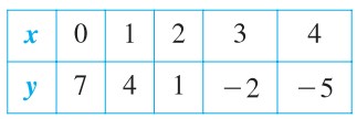
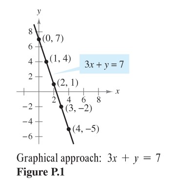
From the table, you can see that $(0,7), (1,4), (2,1), (3,-2), (4,-5)$ are solutions of the original equation $3x+y=7$ . Like many equations, this equation has an infinite nuber of solutions. The sets of all solution point is the graph of the equation, as shown in Figure P1.

Even thought we refer the sketch shown in Figure P1 as the graph of $3x+y=7$ , it really represents only a portion of the graph. The entire graph would extend beyond this page.

In this course, you will study many sketching techniques. The simplest is point plotting. That is, you plot points until the basic shape of the graph seems apparent.

EXAMPLE 1 – Sketching a Graph by Point Plotting

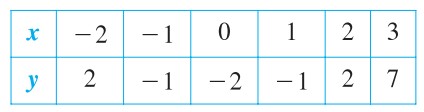
Sketch the graph of $y=x^2-2$

Solution

First construct the table of values.
Calculus 00003
Then plot the points shown in the table
Calculus 00004
Finally, connect the points with a smooth curve as shown in Figure P2.
This graph is a parabola. It is one of the conics you will study later.

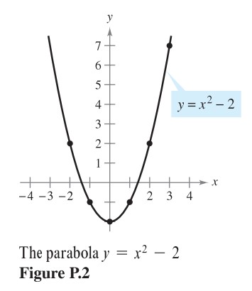
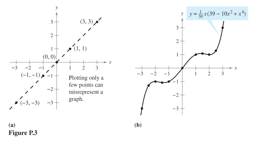
One disadvantage of plotting is that to get a good idea about the shape of a graph, you may need to plot many points. With only a few points, you could badly misrepresent the graph. For instance, suppose that to sketch the graph of

$\displaystyle y=\frac{1}{30} x\left(39-10 x^2+x^4\right)$

you plotted only five points: $(-3,-3),(-1,-1),(0,0),(1,1), \text { and }(3,3)$ , as shown in Figure P3 (a). From these five points, you might conclude that the graph is line. This, however, is not correct. By plotting several more points, you can see that the graph is more complicated, as shown in Figure P3 (b).

Calculus 00005

EXERCISES

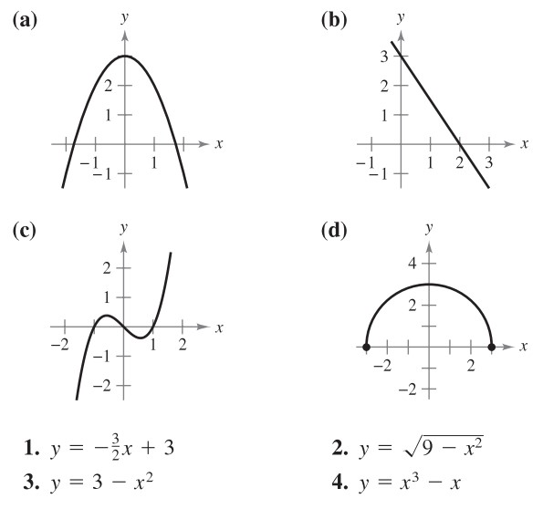
In exercises 1-4, match the equation with its graph. The graphs are labeled (a), (b), (c), and (d).

Calculus 00008

[1, 2, 3, 4]

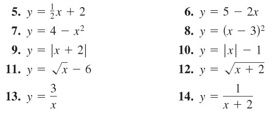
In exercises 5-14, sketch the graph of the equation by point plotting.

Calculus 00009

[5, 6, 7, 8, 9, 10, 11, 12, 13, 14]

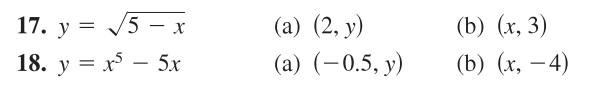
In exercises 17 and 18, use Geogebra to graph the equation. Find the unknown coordinate of each solution point accurate to two decimal places.

Calculus 00010

[17a, 17b, 18a, 18b]

Intercepts of a Graph

Two types of solution points that are specially useful in graphing an equation are those having zero as $x$ – or $y$ -coordinate. Such points are called intercepts because they are the points at which the graph intersects the $x$ – or $y$ -axis.

The point $(a,0)$ is an x-intercept of the graph of an equation if it is a solution point of the equation. To find the $x$ – intercepts of a graph, let $y$ be zero and solve the equation for $x$ .

The point $(0,b)$ is a y-intercept of the graph of an equation if it is a solution point of the equation. To find the $y$ -intercepts of a graph, let $x$ be zero and solve the equation for $y$ .

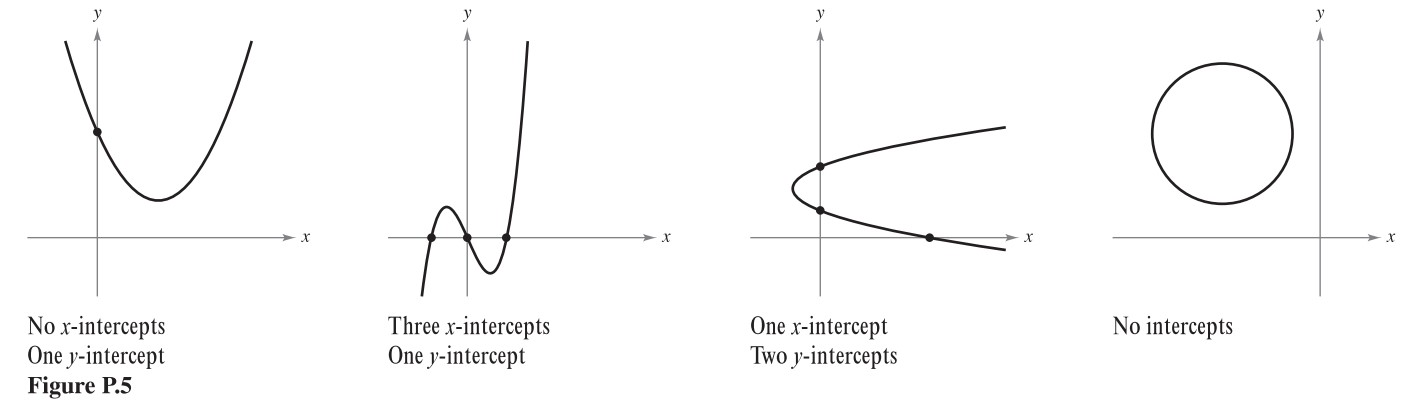
It is possible for a graph to have no intercepts, or it might have several. For instance, consider the graphs shown in Figure P5.

Calculus 00006

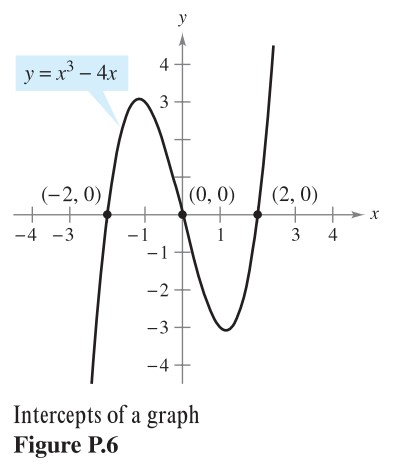
EXAMPLE 2 – Finding x– and y-intercepts

Find the $x$ – and $y$ -intercepts of the graph of $y=x^3-4x$

Solution

To find the $x$ -intercepts, ley $y$ be zero and solve for $x$ .

$\begin{aligned} x^3-4 x & =0 \\ x(x-2)(x+2) & =0 \\ x & =0,2, \text { or }-2 \end{aligned}$

Because this equation has three solutions, you can conclude that the graph has three $x$ -intercepts:

$(0,0),(2,0), \text { and }(-2,0)$

To find the $y$ -intercepts, let $x$ be zero.

Doing this proces $y=0$ . So the $y$ -intercept is $(0,0)$

Calculus 00007

Example 2 uses an analytic approach to finding intercepts. When an analytic approach is not possible, you can use a graphical approach by finding the points at wich the graph intersects the axes. Use a graphing utility to approximate the intercepts.

EXERCISES

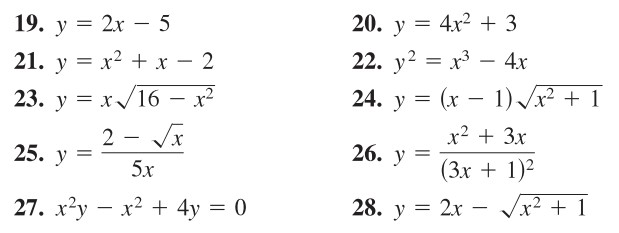
In Exercises 19-28, find any intercepts.

Calculus 00011

[19, 20, 21, 22, 23, 24, 25, 26, 27, 28]

Los

Summary

The Graph of an Equation

EXAMPLE 1 – Sketching a Graph by Point Plotting

Solution

EXERCISES

In exercises 1-4, match the equation with its graph. The graphs are labeled (a), (b), (c), and (d).

In exercises 5-14, sketch the graph of the equation by point plotting.

In exercises 17 and 18, use Geogebra to graph the equation. Find the unknown coordinate of each solution point accurate to two decimal places.

Intercepts of a Graph

EXAMPLE 2 – Finding x– and y-intercepts

Solution

EXERCISES

In Exercises 19-28, find any intercepts.

Deja un comentarioCancelar respuesta